解读CUDA

“既然我可以直接使用 PyTorch，为什么还要费心使用 CUDA 呢?”

PyTorch 是一个机器学习库，它允许在 GPU 上创建、训练和运行高级人工智能模型。在很大程度上，人工智能在过去几年的快速发展都要归功于 PyTorch 的易用性和强大功能。但是，在AI应用的开发过程中，PyTorch 并不总是足够的。例如，Flash Attention将注意力的实现速度提高了10倍，这是通过重新设计 PyTorch 在 CUDA 中实现的。 随着人工智能作为一门学科的成熟，效率变得越来越重要。

人们的共识是模型越大越好。人工智能模型能够被训练和服务的效率越高，它们就能变得越大，也就越有用。尽管 PyTorch 在推动技术进步方面至关重要，但低层 CUDA 仍然是有效实现尖端人工智能的重要工具。此外，PyTorch 使用了 CUDA 与 GPU 接口，所以即使我们正在使用 PyTorch，也可能在底层使用了 CUDA。我们可以在 CUDA 中创建自定义的 PyTorch 功能，CUDA 可以成为一个有用的技能来学习。

那么，如何学习CUDA呢？ 让我们从计算机的体系结构谈起。

1. 计算机的体系结构及一般组成

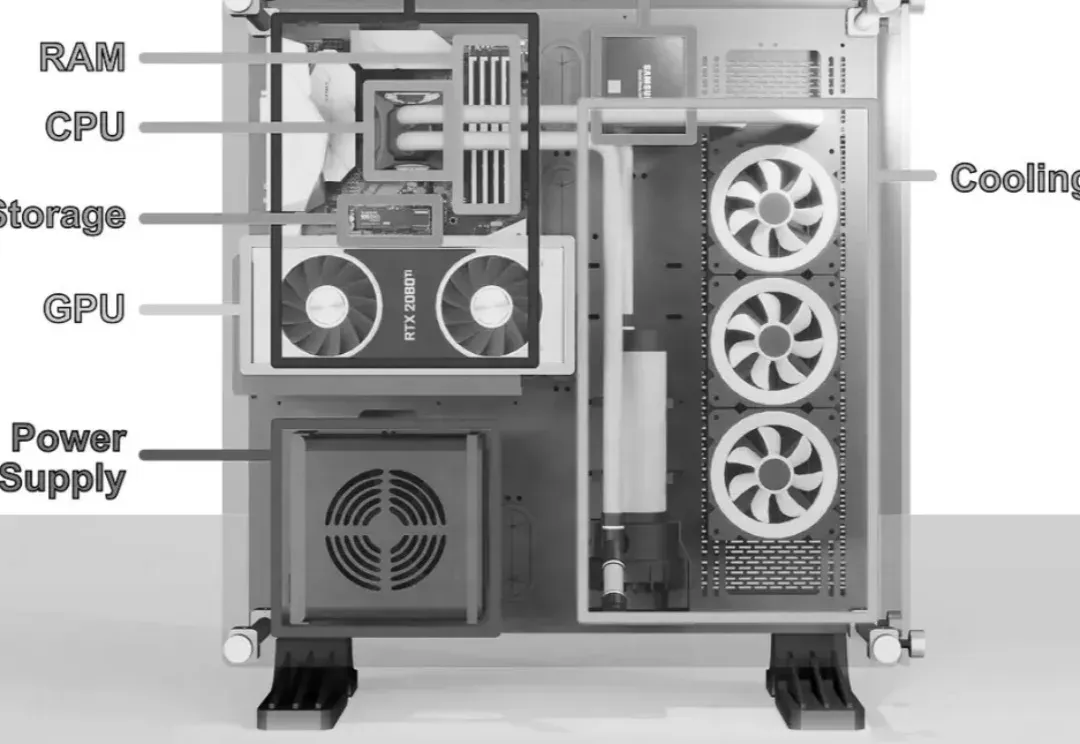
一般地，计算机的构成如下所示：（这让我想起了30多年前，在中关村自己组装计算机的那些日子......)

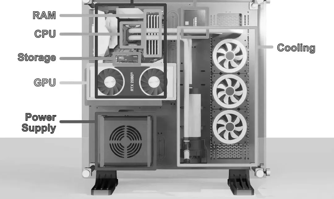
主板是计算机的主干。它本质上是一个大的电路板，可以让计算机的各个部件相互通信。在主板的中间是几乎所有现代计算机的心脏: CPU，或“中央处理器”。CPU 负责执行运行程序所必需的计算，因此是计算机最重要的组成部分之一。

因为中央处理器产生热量，中央处理器通常被一个散热器所覆盖，这就是为什么我们不能在这个渲染中看到它。通常，一个 CPU 看起来像一个金属方块，底部有一串引脚。紧挨着CPU的是RAM，它代表“随机存取存储器”。RAM是CPU的工作存储器，旨在允许快速访问相关信息。

许多计算机的另一个流行组件，是图形处理器(GPU) ，关于GPU的更多内容可以参考《温故知新之GPU计算（在新窗口打开）》一文。游戏玩家喜欢他们的 GPU，通俗说法叫“显卡”， 使用带状电缆连接显卡与主板。在设置中，希望GPU 尽可能接近其他组件，因此它可能会直接安装到 PCI-E 端口。

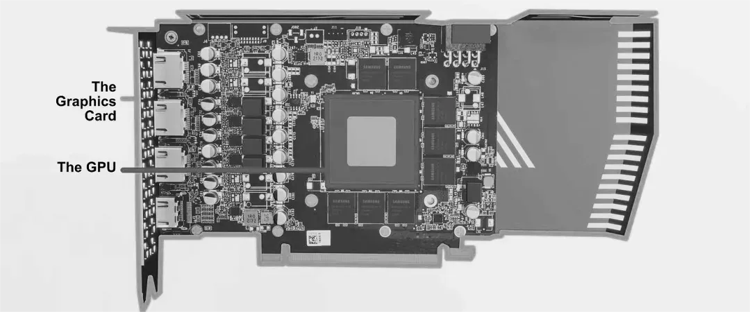
PCI-E，或“ PCI Express”是一组主板上的端口，允许 CPU 与外部设备通信。PCI-E 最常用的是 GPU 的连接，但是 PCI-E 是一个灵活的接口，允许存储设备、专用卡和其他设备连接到计算机。

PCI-E 总线上的组件是计算机核心的“插件”。CPU 和 RAM 在计算机的运行中是至关重要的，而像 GPU 这样的设备就像工具一样，CPU 可以激活它们来做某些事情。即使在低级别的编程中，这种概念仍然是相关的。因此，通常 CPU 和 RAM 被称为“主机”，而 GPU 被称为“设备”。

GPU 有点类似于主机(CPU 和 RAM)。虽然整个显卡通常被称为 GPU，但实际上，术语 GPU 指的是显卡内的一个处理单元。除了 GPU 之外，还有其他的显卡组件，比如 vRAM，它实际上是与 CPU 的 RAM 等价。 显卡设备有一个处理单元和内存，主机（CPU和RAM）也有一个处理单元和内存。设备和主机都拥有彼此独立工作所需的资源，构建同时使用设备和主机的低级应用程序需要对这两个协同工作的实体进行编程。

如果你希望了解计算机的历史，推荐阅读张银奎老师的《软件简史》一书——

既然GPU与CPU如此类似，为什么需要对GPU进行编程呢？ 使用CPU 有什么不足么？

2. CPU 和 GPU

CPU 是由“核心（core）”组成的。核心是设计用来快速完成基本数学运算的电路。虽然很简单，但是核心所能做的数学运算是基础性的，并且结合许多简单的计算可以产生几乎任何可以想象的数学运算。一个现代的 CPU 有多个核心，这样的 CPU 可以同时处理多个事情。中央处理器也有不同类型的内存(称为缓存) ，这是为了加快 CPU 的速度。

CPU 的整个思想就是尽可能快地运行一个程序，它可以被概念化为一个操作列表。虽然 CPU 可以并行处理(称为多线程处理) ，但 CPU 的主要重点是尽可能快地进行背靠背的计算。因此，CPU 的每个核心都被设计成尽可能快地完成每个操作。这种方法对于许多应用程序至关重要。有些计算只是需要一个接一个地进行，而要更快地进行这些计算，唯一的方法就是尽可能快地完成每一步。但是，有些应用程序可以并行化处理。

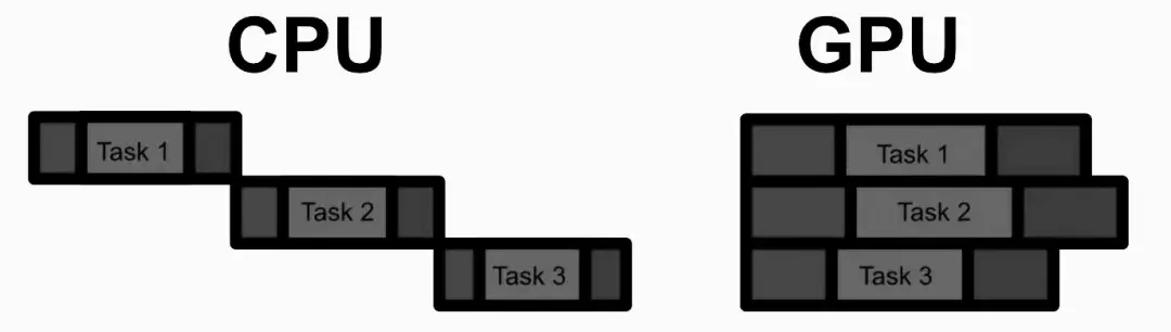
GPU 的思想不是优化单个计算，而是优化批量执行许多计算。一般来说，在给定的计算量时 GPU 比 CPU 慢得多，因此只有当有足够的计算可以并行运行时，GPU 才会真正发光。但是，当应用到合适的问题上时，GPU 可以比 CPU 快100倍甚至1000倍。

在并行计算方面，GPU 与 CPU 有两个主要的不同点:

• GPU 比 CPU 拥有更多的核心，但是这些核心的能力较差。这意味着 GPU 可以同时进行更多的计算，但是这些计算通常比较慢。
• GPU 比 CPU 拥有更多的核心，但是这些核心的能力较差。这意味着 GPU 可以同时进行更多的计算，但是这些计算通常比较慢。

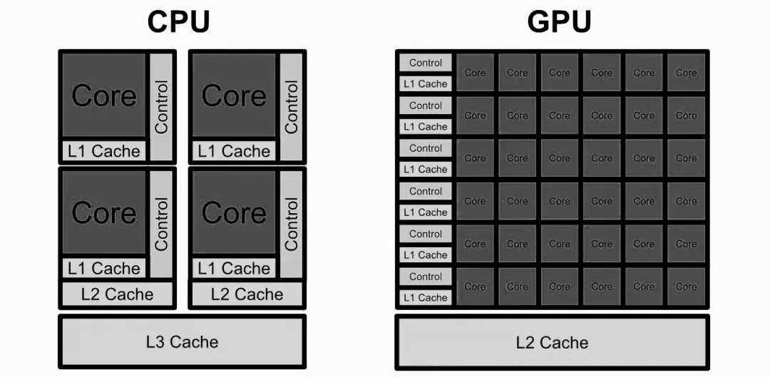
由于人工智能基本上是通过一系列简单的、或多或少独立的计算完成的，人工智能模型是 GPU 的完美用例。

3. 面向GPU的编程框架-CUDA

CUDA（Compute Unified Device Architecture）是 NVIDIA 的并行计算平台。CUDA 本质上是一套用于构建在 CPU 上运行的应用程序的工具，可以对 GPU 进行并行计算。

有一个方便的 Jupiter 扩展，可以编译和运行 CUDA 代码，就像是一个正常的代码块。这使得 Jupiter 可以连接到 NVIDIA 的 CUDA 编译器 nvcc。

!pip install nvcc4jupyter

%load_ext nvcc4jupyter

3.1 启动和配置

让我们从永远的Hello world 开始：

%%cuda

//we'll cover what all this stuff means soon

#include <stdio.h>

__global__ void hello(){

printf("Hello from block: %u, thread: %u\n", blockIdx.x, threadIdx.x);

}

__host__ int main(){

hello<<<2, 2>>>();

cudaDeviceSynchronize();

}

CUDA 的第一个基本思想是kernel，基本上是一个在 GPU 上并行运行多次的函数。在 CUDA 中，我们在函数定义之前用 _ _ global _ _ 关键字定义一个内核。我们还可以使用 _ _ host _ _ 关键字定义在 CPU 上运行的代码。 因为这是 C + +程序 ，所以首先执行的是 main 函数，这个函数在 CPU (也就是主机)上。然后，在 CPU 上，调用的第一行代码是hello < < < 2,2 > > > ()，这称为启动配置，并在 GPU 上启动 CUDA 的kernel hello。

在 CUDA 中，并行作业被组织成“线程”，其中线程是能够并行工作程序的一部分。我们可以在 GPU 上对多个线程进行后台处理，它们可以一起工作来完成某些任务。这些线程存在于所谓的“线程块”中。在现代 GPU 上，每个线程块可以有1024个线程。同一个线程块中的线程在 vRAM 中共享相同的地址空间(相当于 GPU 中的 RAM) ，因此它们能够在相同的数据上协同工作。虽然每个块只能有1024个线程，但是在 GPU 上可以有成吨的线程块排队等待。

大多数 GPU 具有一次执行多个线程块的资源。一个 GPU 可能一次只能执行两个线程块，另一个可能能够执行十八个。这意味着相同的 CUDA 代码可以利用大型和小型 GPU。

在helloword中，我们定义了将在启动配置中使用多少线程和线程块。在<<<>>>中，我们将线程块的数量指定为第一个参数，将每个块的线程数量指定为第二个参数。因为kernel 是在 GPU 上运行的，为了将打印结果重新打印到 CPU 上以便在Jupiter上显示，使用 cudaDeviceSynchronize 等待 GPU 上的所有线程完成，然后打印输出。

当运行kernel时，CUDA 会自动创建一些方便的变量。两个非常重要的变量是 blockIdx 和 threadIdx，可以使用这些变量来了解当前正在运行的线程块和线程。线程块可以组织多达三个维度的线程，这意味着 blockIdx 和 threadIdx 具有 x、 y 和 z 属性。

%%cuda

#include <stdio.h>

__global__ void hello() {

printf("Hello from block: (%u, %u, %u), thread: (%u, %u, %u)\n",

blockIdx.x, blockIdx.y, blockIdx.z,

threadIdx.x, threadIdx.y, threadIdx.z);

}

int main() {

// Define the dimensions of the grid and blocks

dim3 gridDim(2, 2, 2); // 2x2x2 grid of blocks

dim3 blockDim(2, 2, 2); // 2x2x2 grid of threads per block

// Launch the kernel

hello<<<gridDim, blockDim>>>();

// Wait for GPU to finish before accessing on host

cudaDeviceSynchronize();

return 0;

}

也就是说，CUDA 允许构建最多三维的计算网格，并通过 lockIdx 和 threadIdx 通知线程它在该网格中的位置。

3.2 设备与主机间的通信

为了将数据发送到 GPU，可以首先使用 cudaMalloc 在 vRAM 上保留一些位置，使用 cudaMemcpy 在 RAM 和 vRAM 之间复制数据，当在 GPU 上完成操作时，我们可以使用 cudaFree 让 GPU 知道我们不再需要 vRAM 中的数据。在将数据发送到 vRAM 之后，我们可以在该数据上运行kernel，然后将结果复制回 RAM，从而有效地使用 GPU 进行计算。

%%cuda

#include <iostream>

#include <cuda.h>

using namespace std;

// Defining the kernel

__global__ void addIntsCUDA(int *a, int *b) {

a[0] += b[0];

}

// Running main on host, which triggers the kernel

int main() {

// Host values

int a = 1, b = 2;

//printing expression

cout << a << " + " << b <<" = ";

// Device pointers (GPU)

int *d_a, *d_b;

// Allocating memory on the device (GPU)

cudaMalloc(&d_a, sizeof(int));

cudaMalloc(&d_b, sizeof(int));

// Copying values from the host (CPU RAM) to the device (GPU)

cudaMemcpy(d_a, &a, sizeof(int), cudaMemcpyHostToDevice);

cudaMemcpy(d_b, &b, sizeof(int), cudaMemcpyHostToDevice);

// Calling the kernel to add the two values at the two pointer locations.

addIntsCUDA<<<1, 1>>>(d_a, d_b);

// The addition function overwrites the a pointer with the sum. Thus

// this copies the result.

cudaMemcpy(&a, d_a, sizeof(int), cudaMemcpyDeviceToHost);

//printing result

cout << a << endl;

//freeing memory.

cudaFree(d_a);

cudaFree(d_b);

return 0;

}

这段代码向 GPU 发送两个值，使用 GPU 将这些数字相加，然后将结果返回到 RAM 并打印出结果。基本上，可以将 RAM 和 vRAM 都看作是一个大数组。当代码int a = 1，b = 2;在 CPU 上被触发时，将在 RAM 中分配两个地址来存储这两个值。当我们调用 & a 或 & b 时，我们得到的是这些值的地址，而不是这些值本身。通过运行 CudaMalloc，现在已经在 vRAM 上分配了底座以及 RAM 上的指针，告诉我们这些地址在 vRAM 上的位置。

cudaMemcpy 指定了从主机复制到设备，这将导致将 a 和 b 的值复制到设备。

GPU 不知道 CPU 是否接近程序的末尾，所以 GPU 上的值会一直保持在那里，直到应用程序执行完毕，需要cudaFree 来释放vRAM。

3.3 在 GPU 上并行处理 的CPU 程序

下面是一个示例，试图为一组点中的每个3D 点找到最接近的其他点，最终结果应该是一个列表，其中列表中的 i 点中的值应该是 i 点最接近的点的索引。所以，如果有三个点，点1最接近点3点2最接近点3点3最接近点2输出看起来像[3,3,2]。下面是 CPU 上的实现:

%%cuda

#include <iostream>

#include <ctime>

#include <cuda.h>

#include <cuda_runtime.h>

#include <device_launch_parameters.h>

using namespace std;

//brute force approach to finding which point

void findClosestCPU(float3* points, int* indices, int count) {

// Base case, if there's 1 point don't do anything

if(count <=1) return;

// Loop through every point

for (int curPoint = 0; curPoint < count; curPoint++) {

// set as close to the largest float possible

float distToClosest = 3.4028238f ;

// See how far it is from every other point

for (int i = 0; i < count; i++) {

// Don't check distance to itself

if(i == curPoint) continue;

float dist_sqr = (points[curPoint].x - points[i].x) *

(points[curPoint].x - points[i].x) +

(points[curPoint].y - points[i].y) *

(points[curPoint].y - points[i].y) +

(points[curPoint].z - points[i].z) *

(points[curPoint].z - points[i].z);

if(dist_sqr < distToClosest) {

distToClosest = dist_sqr;

indices[curPoint] = i;

}

}

}

}

int main(){

//defining parameters

const int count = 10000;

int* indexOfClosest = new int[count];

float3* points = new float3[count];

//defining random points

for (int i = 0; i < count; i++){

points[i].x = (float)(((rand()%10000))-5000);

points[i].y = (float)(((rand()%10000))-5000);

points[i].z = (float)(((rand()%10000))-5000);

}

long fastest = 1000000000;

cout << "running brute force nearest neighbor on the CPU..."<<endl;

for (int i = 0; i <= 10; i++){

long start = clock();

findClosestCPU(points, indexOfClosest, count);

double duration = ( clock() - start ) / (double) CLOCKS_PER_SEC;

cout << "test " << i << " took " << duration << " seconds" <<endl;

}

return 0;

}

要在 GPU 上并行化这段代码，我们需要获取 vRAM 上的地址，然后在 GPU 上以kernel的形式启动findClosest。

%%cuda

#include <iostream>

#include <ctime>

#include <cuda.h>

#include <cuda_runtime.h>

#include <device_launch_parameters.h>

using namespace std;

// Brute force implementation, parallelized on the GPU

__global__ void findClosestGPU(float3* points, int* indices, int count) {

if (count <= 1) return;

int idx = threadIdx.x + blockIdx.x * blockDim.x;

if (idx < count) {

float3 thisPoint = points[idx];

float smallestSoFar = 3.40282e38f;

for (int i = 0; i < count; i++) {

if (i == idx) continue;

float dist_sqr = (thisPoint.x - points[i].x) *

(thisPoint.x - points[i].x) +

(thisPoint.y - points[i].y) *

(thisPoint.y - points[i].y) +

(thisPoint.z - points[i].z) *

(thisPoint.z - points[i].z);

if (dist_sqr < smallestSoFar) {

smallestSoFar = dist_sqr;

indices[idx] = i;

}

}

}

}

int main() {

// Defining parameters

const int count = 10000;

int* h_indexOfClosest = new int[count];

float3* h_points = new float3[count];

// Defining random points

for (int i = 0; i < count; i++) {

h_points[i].x = (float)(((rand() % 10000)) - 5000);

h_points[i].y = (float)(((rand() % 10000)) - 5000);

h_points[i].z = (float)(((rand() % 10000)) - 5000);

}

// Device pointers

int* d_indexOfClosest;

float3* d_points;

// Allocating memory on the device

cudaMalloc(&d_indexOfClosest, sizeof(int) * count);

cudaMalloc(&d_points, sizeof(float3) * count);

// Copying values from the host to the device

cudaMemcpy(d_points, h_points, sizeof(float3) * count, cudaMemcpyHostToDevice);

int threads_per_block = 64;

cout << "Running brute force nearest neighbor on the GPU..." << endl;

for (int i = 1; i <= 10; i++) {

long start = clock();

findClosestGPU<<<(count / threads_per_block) + 1, threads_per_block>>>(d_points, d_indexOfClosest, count);

cudaDeviceSynchronize();

// Copying results from the device to the host

cudaMemcpy(h_indexOfClosest, d_indexOfClosest, sizeof(int) * count, cudaMemcpyDeviceToHost);

double duration = (clock() - start) / (double)CLOCKS_PER_SEC;

cout << "Test " << i << " took " << duration << " seconds" << endl;

}

// Freeing device memory

cudaFree(d_indexOfClosest);

cudaFree(d_points);

// Freeing host memory

delete[] h_indexOfClosest;

delete[] h_points;

return 0;

}

在这段代码中， 我们创建了一堆需要排序的随机点，将点从 RAM 复制到 vRAM，然后我们运行kernel。kernel本身只需要一些修改，就可以将其从 CPU 转换为 GPU。

我们可以为每个线程分配一个单独的地址，指定为 idx。我们可以通过从所有的线程块中计算当前正在执行的线程来做到这一点。我们可以使用这个惟一的 id 将每个线程分配给一个特定的点。所以线程0负责找到最接近点0的点，线程50负责找到最接近点50的点，等等。通常线程太多，因为可能没有足够的点来填充最后一个线程块，所以我们只计算有效的 idx 值。一旦kernel执行完毕，所有的值都更新了，我们就可以将它们复制回主机，然后对它们做任何想做的事情。

3.4 NVIDIA Profiler

在 CUDA 中实现复杂的并行程序时，了解哪些类型的操作对性能影响最大是有用的。

我们可以使用%% writefile findclosestgpu.cu 将 CUDA 代码块写成文本文件，而不是在代码块的顶部调用%% CUDA。然后，可以使用 nvprof 来分析用于执行 CUDA 代码的计算：!nvprof ./findClosestGPU.out。一般来说，在进行 CUDA 编程时，大部分时间都花在优化内存和设备间通信上，而不是计算本身。

4. 基于CUDA 的神经网络编程

CUDA，从硬核低级开发人员的角度来看，实际上是一个高级编程工具。

从定义一个示例工程开始，我们将建立一个数据结构shape来定义神经网络中的数据，为 CUDA 中的异常错误建立一个抽象类来帮助调试，建立一个矩阵的抽象以及二元交叉熵。一旦设置完成，我们将构建一些组成模型本身的类，模型的层通用类以及线性层的实现、 sigmoid 和 ReLu 激活函数。最后，构建、训练并测试这个模型。

4.1 一个简单的C++ 工程

定义头文件：

%%writefile someClass.hh

// this is used so, if someClass gets imported multiple times across several

// documents, it only actually gets imported once.

#pragma once

class ClassWithFunctionality {

// defining private things for internal use

private:

// defining private data

int someValue;

int anotherValue;

// defining private functions

void privateFunction1();

void privateFunction2();

// defining things accessible outside the object

public:

// defining public data

int somePublicValue;

int someOtherPublicValue;

// defining public functions

ClassWithFunctionality(int constructorInput);

void doSomething1();

void doSomething2();

};

然后是具体的实现文件：

%%writefile someClass.cu

#include "someClass.hh"

// defining constructor

ClassWithFunctionality::ClassWithFunctionality(int constructorInput)

: someValue(constructorInput), anotherValue(2), somePublicValue(3), someOtherPublicValue(4)

{}

void ClassWithFunctionality::doSomething1() {

return;

}

void ClassWithFunctionality::doSomething2() {

return;

}

void ClassWithFunctionality::privateFunction1() {

return;

}

void ClassWithFunctionality::privateFunction2() {

return;

}

虽然已经有了头文件和 CUDA 文件，但实际上不能运行它，因为没有 main 函数。快速创建一个 main 函数，以便测试我们的功能。

%%writefile main.cu

#include <iostream>

#include "someClass.hh"

// testing SomeClass

int main(void) {

ClassWithFunctionality example(3);

std::cout << "it works!" << std::endl;

return 0;}

然后，要实编译这段代码，运行它，将输出保存到一个文件中，打印出这个文件。

!nvcc someClass.cu main.cu -o outputFile.out

!./outputFile.out

4.2 工具类

4.2.1 shape

AI大量使用2D 矩阵，我们可以定义一个名为shape的数据结构，使用它来跟踪2D 矩阵的大小。

%%writefile shape.hh

#pragma once

struct Shape {

size_t x, y;

Shape(size_t x = 1, size_t y = 1);

};

%%writefile shape.cu

#include "shape.hh"

Shape::Shape(size_t x, size_t y) :

x(x), y(y)

{ }

%%writefile main.cu

#include "shape.hh"

#include <iostream>

#include <stdio.h>

using namespace std;

//testing

int main( void ) {

Shape shape = Shape(100, 200);

cout << "shape x: " << shape.x << ", shape y: " << shape.y << endl;

}

!nvcc shape.cu main.cu -o shape.out

!./shape.out

4.2.2 NNException

如果GPU上发生问题，可能需要一段时间才能将问题传播回CPU。这可能会使调试CUDA程序变得困难。为了缓解这种情况，可以使用cudaGetLastError（）来检查GPU上的最新错误。NNException是一个围绕cudaGetLastError构建的轻量级封装，它允许我们在整个代码中检查GPU上是否存在错误。

%%writefile nn_exception.hh

#pragma once

#include <exception>

#include <iostream>

class NNException : std::exception {

private:

const char* exception_message;

public:

NNException(const char* exception_message) :

exception_message(exception_message)

{ }

virtual const char* what() const throw()

{

return exception_message;

}

static void throwIfDeviceErrorsOccurred(const char* exception_message) {

cudaError_t error = cudaGetLastError();

if (error != cudaSuccess) {

std::cerr << error << ": " << exception_message;

throw NNException(exception_message);

}

}

};

%%writefile main.cu

//With error handling

#include "nn_exception.hh"

#include <cuda_runtime.h>

int main() {

// Allocate memory on the GPU

float* d_data;

cudaError_t error = cudaMalloc((void**)&d_data, 100 * sizeof(float));

// Check for CUDA errors and throw an exception if any

try {

NNException::throwIfDeviceErrorsOccurred("Failed to allocate GPU memory");

} catch (const NNException& e) {

std::cerr << "Caught NNException: " << e.what() << std::endl;

return -1; // Return an error code

}

// Free the GPU memory

error = cudaFree(d_data);

// Check for CUDA errors again

try {

NNException::throwIfDeviceErrorsOccurred("Failed to free GPU memory");

} catch (const NNException& e) {

std::cerr << "Caught NNException: " << e.what() << std::endl;

return -1; // Return an error code

}

std::cout << "CUDA operations completed successfully" << std::endl;

return 0; // Return success

}

!nvcc main.cu shape.cu -o nnexception.out

!./nnexception.out

4.2.3 矩阵

这个类抽象了设备和主机之间的一些通信，允许在内存位置之间轻松地传递值矩阵：

1. 在 CPU 和 GPU 上为矩阵分配的内存
2. 将数据从 CPU RAM 复制到 GPU VRAM
3. 将数据从 GPU VRAM 复制到 CPU RAM
4. 像数组一样对矩阵进行索引

%%writefile matrix.hh

#pragma once

#include "shape.hh"

#include <memory>

class Matrix {

private:

bool device_allocated;

bool host_allocated;

void allocateCudaMemory();

void allocateHostMemory();

public:

Shape shape;

std::shared_ptr<float> data_device;

std::shared_ptr<float> data_host;

Matrix(size_t x_dim = 1, size_t y_dim = 1);

Matrix(Shape shape);

void allocateMemory();

void allocateMemoryIfNotAllocated(Shape shape);

void copyHostToDevice();

void copyDeviceToHost();

float& operator[](const int index);

const float& operator[](const int index) const;

};

%%writefile matrix.cu

#include "matrix.hh"

#include "nn_exception.hh"

using namespace std;

Matrix::Matrix(size_t x_dim, size_t y_dim) :

shape(x_dim, y_dim), data_device(nullptr), data_host(nullptr),

device_allocated(false), host_allocated(false)

{ }

Matrix::Matrix(Shape shape) :

Matrix(shape.x, shape.y)

{ }

void Matrix::allocateCudaMemory() {

if (!device_allocated) {

float* device_memory = nullptr;

cudaMalloc(&device_memory, shape.x * shape.y * sizeof(float));

NNException::throwIfDeviceErrorsOccurred("Cannot allocate CUDA memory for Tensor3D.");

data_device = std::shared_ptr<float>(device_memory,

[&](float* ptr){ cudaFree(ptr); });

device_allocated = true;

}

}

void Matrix::allocateHostMemory() {

if (!host_allocated) {

data_host = std::shared_ptr<float>(new float[shape.x * shape.y],

[&](float* ptr){ delete[] ptr; });

host_allocated = true;

}

}

void Matrix::allocateMemory() {

allocateCudaMemory();

allocateHostMemory();

}

void Matrix::allocateMemoryIfNotAllocated(Shape shape) {

if (!device_allocated && !host_allocated) {

this->shape = shape;

allocateMemory();

}

}

void Matrix::copyHostToDevice() {

if (device_allocated && host_allocated) {

cudaMemcpy(data_device.get(), data_host.get(), shape.x * shape.y * sizeof(float), cudaMemcpyHostToDevice);

NNException::throwIfDeviceErrorsOccurred("Cannot copy host data to CUDA device.");

}

else {

throw NNException("Cannot copy host data to not allocated memory on device.");

}

}

void Matrix::copyDeviceToHost() {

if (device_allocated && host_allocated) {

cudaMemcpy(data_host.get(), data_device.get(), shape.x * shape.y * sizeof(float), cudaMemcpyDeviceToHost);

NNException::throwIfDeviceErrorsOccurred("Cannot copy device data to host.");

}

else {

throw NNException("Cannot copy device data to not allocated memory on host.");

}

}

float& Matrix::operator[](const int index) {

return data_host.get()[index];

}

const float& Matrix::operator[](const int index) const {

return data_host.get()[index];

}

%%writefile main.cu

#include <iostream>

#include "matrix.hh"

#include "nn_exception.hh"

int main() {

// Create a Matrix object with dimensions 10x10

Matrix matrix(10, 10);

// Allocate memory on both host and device

matrix.allocateMemory();

std::cout << "Memory allocated on host and device." << std::endl;

// Initialize host data

for (size_t i = 0; i < 100; ++i) {

matrix[i] = static_cast<float>(i);

}

std::cout << "Host data initialized." << std::endl;

// Copy data from host to device

matrix.copyHostToDevice();

std::cout << "Data copied from host to device." << std::endl;

// Clear host data

for (size_t i = 0; i < 100; ++i) {

matrix[i] = 0.0f;

}

std::cout << "Host data cleared." << std::endl;

// Copy data back from device to host

matrix.copyDeviceToHost();

std::cout << "Data copied from device to host." << std::endl;

// Verify the data

bool success = true;

for (size_t i = 0; i < 100; ++i) {

if (matrix[i] != static_cast<float>(i)) {

success = false;

break;

}

}

if (success) {

std::cout << "Test passed: Data verification successful." << std::endl;

} else {

std::cout << "Test failed: Data verification unsuccessful." << std::endl;

}

return 0;

}

!nvcc main.cu matrix.cu shape.cu -o matrix.out

!./matrix.out

关于深度学习中涉及的各种数学知识，可以参考笔者翻译的《深度学习的黑箱》一书——

4.3 定义损失函数

损失函数告诉模型它在输出预测时的错误程度，根据错误的程度来更新模型，详见《神经网络中常见的激活函数（在新窗口打开）》一文。损失函数的一个非常重要的特征是不仅要计算出一个模型的错误程度，而且还要计算出哪些输出会更好。这是必要的，以便我们可以找出如何更新模型参数，以产生更好的输出。例如，二元交叉熵如下所示：

在cuda中，我们可以定义一个这样的类：

%%writefile bce_cost.hh

#pragma once

#include "matrix.hh"

class BCECost {

public:

float cost(Matrix predictions, Matrix target);

Matrix dCost(Matrix predictions, Matrix target, Matrix dY);

};

为了实现二元交叉熵建模，我们只需要实现两个函数:

1. 一个计算给定输出列表的预测损失
2. 一个用来计算损失的导数。因此，实质上，“这个预测应该更大，这个预测应该更小”的列表。

我们可以将这些函数作为可以在 GPU 上执行的kernel来实现，这样就可以并行处理这些计算。

__global__ void binaryCrossEntropyCost(float* predictions, float* target,

int size, float* cost) {

int index = blockIdx.x * blockDim.x + threadIdx.x;

if (index < size) {

// Clamp predictions to avoid log(0)

float pred = predictions[index];

pred = fmaxf(fminf(pred, 1.0f - 1e-7), 1e-7);

float partial_cost = target[index] * logf(pred)

+ (1.0f - target[index]) * logf(1.0f - pred);

atomicAdd(cost, - partial_cost / size);

}

}

计算损失导数的kernel为：

__global__ void dBinaryCrossEntropyCost(float* predictions, float* target, float* dY,

int size) {

int index = blockIdx.x * blockDim.x + threadIdx.x;

if (index < size) {

// Clamp predictions to avoid division by zero

float pred = predictions[index];

pred = fmaxf(fminf(pred, 1.0f - 1e-7), 1e-7);

dY[index] = -1.0 * (target[index] / pred - (1 - target[index]) / (1 - pred));

}

}

内核中维护不同的一个指针来分别指示存储输出的位置、 float * Cost 和 float * dY。损失函数简单地将二元交叉熵函数应用于所有点，并将它们在损失位置上相加。二元交叉熵函数的导数遍历所有点，计算该点的导数，并存储该值在 dY 中，表明应该是高还是低的值，都是由 BCECost 类的 Cost 和 dCost 方法调用的。

//cost (or loss)

float BCECost::cost(Matrix predictions, Matrix target) {

assert(predictions.shape.x == target.shape.x);

float* cost;

cudaMallocManaged(&cost, sizeof(float));

*cost = 0.0f;

dim3 block_size(256);

dim3 num_of_blocks((predictions.shape.x + block_size.x - 1) / block_size.x);

binaryCrossEntropyCost<<<num_of_blocks, block_size>>>(predictions.data_device.get(),

target.data_device.get(),

predictions.shape.x, cost);

cudaDeviceSynchronize();

NNException::throwIfDeviceErrorsOccurred("Cannot compute binary cross entropy cost.");

float cost_value = *cost;

cudaFree(cost);

return cost_value;

}

//derivative of cost (aka derivative of loss)

Matrix BCECost::dCost(Matrix predictions, Matrix target, Matrix dY) {

assert(predictions.shape.x == target.shape.x);

dim3 block_size(256);

dim3 num_of_blocks((predictions.shape.x + block_size.x - 1) / block_size.x);

dBinaryCrossEntropyCost<<<num_of_blocks, block_size>>>(predictions.data_device.get(),

target.data_device.get(),

dY.data_device.get(),

predictions.shape.x);

NNException::throwIfDeviceErrorsOccurred("Cannot compute derivative for binary cross entropy.");

return dY;

}

这两个函数的行为通常相似，Cost 创建它自己的值并返回它，而 dCost 期望它的输出 dY 作为输入并修改它。

%%writefile main.cu

#include <iostream>

#include <vector>

#include "matrix.hh"

#include "bce_cost.hh"

#include "nn_exception.hh"

// Helper function to initialize a Matrix with data

void initializeMatrix(Matrix& matrix, const std::vector<float>& data) {

for (size_t i = 0; i < data.size(); ++i) {

matrix[i] = data[i];

}

matrix.copyHostToDevice();

}

int main() {

// Define the size of the data

const int size = 10;

// Create predictions and target data

std::vector<float> predictions_data = {0.1, 0.2, 0.3, 0.4, 0.5, 0.6, 0.7, 0.8, 0.9, 0.95};

std::vector<float> target_data = {0, 0, 1, 0, 1, 0, 1, 1, 1, 0};

// Create Matrix objects for predictions and targets

Matrix predictions(size, 1);

Matrix target(size, 1);

predictions.allocateMemory();

target.allocateMemory();

// Initialize matrices with data

initializeMatrix(predictions, predictions_data);

initializeMatrix(target, target_data);

// Compute the binary cross-entropy cost

BCECost bce_cost;

float cost_value = bce_cost.cost(predictions, target);

std::cout << "Binary Cross-Entropy Cost: " << cost_value << std::endl;

// Compute the gradient of the binary cross-entropy cost

Matrix dY(size, 1);

dY.allocateMemory();

Matrix dCost_matrix = bce_cost.dCost(predictions, target, dY);

dCost_matrix.copyDeviceToHost();

// Print the gradient values

std::cout << "Gradient of Binary Cross-Entropy Cost: ";

for (int i = 0; i < size; ++i) {

std::cout << dCost_matrix[i] << " ";

}

std::cout << std::endl;

return 0;

}

!nvcc main.cu matrix.cu shape.cu bce_cost.cu -o bce.out

!./bce.out

注意，当预测值大于目标值时，导数的结果是正的。当预测值小于目标值时，导数为负。此外，预测误差越大，导数的大小(正或负)就越大。这种一般性质是至关重要的，因为它允许我们基于模型误差的方式以正确的方式更新模型。

4.4 定义模型

示例问题是，给定一个二维空间中的点，模型应该预测它是在左下角还是右上角象限(输出为0) ，或者在右下角还是左上角象限(输出为1)。具体来说，我们将使用这样一个神经网络:

NeuralNetwork nn;

nn.addLayer(new LinearLayer("linear_1", Shape(2, 30)));

nn.addLayer(new ReLUActivation("relu_1"));

nn.addLayer(new LinearLayer("linear_2", Shape(30, 1)));

nn.addLayer(new SigmoidActivation("sigmoid_output"));

线性层由一系列的节点和边组成，每个边有一定的权重，每个节点有一定的偏置。当值通过线性层时，值乘以权重，并加上偏置。

激活函数是旨在为线性层增加非线性的特性。通过向线性层中注入像 ReLU 这样的非线性函数，它允许线性网络学习更复杂的关系。关于激活函数可以参考《神经网络中常见的激活函数（在新窗口打开）》。Sigmoid 类似于 relU，经常被用作概率输出的激活函数。我们将使用这个函数来创建最终输出。

为了简化问题，这里创建一个名为 NNLayer 的抽象类，所有层都将继承它。

%%writefile nn_layer.hh

#pragma once

#include <iostream>

#include "matrix.hh"

class NNLayer {

protected:

std::string name;

public:

virtual ~NNLayer() = 0;

virtual Matrix& forward(Matrix& A) = 0;

virtual Matrix& backprop(Matrix& dZ, float learning_rate) = 0;

std::string getName() { return this->name; };

};

inline NNLayer::~NNLayer() {}

每个 NNLayer 将实现两个关键的函数:

• forward：给定一个输入到网络中，该层将计算值传递给下一层，最终产生一个预测
• backprop：假设损失函数的导数指示的是一个更好的输出，这个函数通知前一层它应该如何更新参数以产生一个更好的输出。

那么，线性层正向传播的 CUDA kernel 为

//in this code W is the weight matrix, A is the input, Z is the output

//and b is the bias, then there are dimensions for the weight matrix

//and the input matrix.

__global__ void linearLayerForward( float* W, float* A, float* Z, float* b,

int W_x_dim, int W_y_dim,

int A_x_dim, int A_y_dim) {

int row = blockIdx.y * blockDim.y + threadIdx.y;

int col = blockIdx.x * blockDim.x + threadIdx.x;

int Z_x_dim = A_x_dim;

int Z_y_dim = W_y_dim;

float Z_value = 0;

if (row < Z_y_dim && col < Z_x_dim) {

for (int i = 0; i < W_x_dim; i++) {

Z_value += W[row * W_x_dim + i] * A[i * A_x_dim + col];

}

Z[row * Z_x_dim + col] = Z_value + b[row];

}

}

线性层也需要一个反向传播的核，所以如果我们知道线性层的输出应该如何变化，我们就可以算出线性网络的输入应该如何变化。

//in this code W is the weight matrix, A is the input, dZ is the output

//of the linear layer should change, dA is how the input of the linear

//layer should change, then there are dimensions for the weight matrix

//and the input matrix.

__global__ void linearLayerBackprop(float* W, float* dZ, float *dA,

int W_x_dim, int W_y_dim,

int dZ_x_dim, int dZ_y_dim) {

int col = blockIdx.x * blockDim.x + threadIdx.x;

int row = blockIdx.y * blockDim.y + threadIdx.y;

// W is treated as transposed

int dA_x_dim = dZ_x_dim;

int dA_y_dim = W_x_dim;

float dA_value = 0.0f;

if (row < dA_y_dim && col < dA_x_dim) {

for (int i = 0; i < W_y_dim; i++) {

dA_value += W[i * W_x_dim + row] * dZ[i * dZ_x_dim + col];

}

dA[row * dA_x_dim + col] = dA_value;

}

}

这个计算非常直观。如果输出 dZ 应该变大，那么输入应该变大 dZ 乘以连接输入和输出的权重。输入和输出之间的线性关系，其中线的斜率是权重。输入中的变化是所有连接输出中加权变化的总和，如 for 循环中所示。

为了更新模型的参数，可以创建另外两个kernel。一个用来更新模型的权重，另一个用来更新偏置。

//in this code W is the weight matrix, A is the input, dZ is the output

//of the linear layer should change, dA is how the input of the linear

//layer should change, then there are dimensions for the weight matrix

//and the input matrix.

__global__ void linearLayerUpdateWeights( float* dZ, float* A, float* W,

int dZ_x_dim, int dZ_y_dim,

int A_x_dim, int A_y_dim,

float learning_rate) {

int col = blockIdx.x * blockDim.x + threadIdx.x;

int row = blockIdx.y * blockDim.y + threadIdx.y;

// A is treated as transposed

int W_x_dim = A_y_dim;

int W_y_dim = dZ_y_dim;

float dW_value = 0.0f;

if (row < W_y_dim && col < W_x_dim) {

for (int i = 0; i < dZ_x_dim; i++) {

dW_value += dZ[row * dZ_x_dim + i] * A[col * A_x_dim + i];

}

W[row * W_x_dim + col] = W[row * W_x_dim + col] - learning_rate * (dW_value / A_x_dim);

}

}

//in this code W is the weight matrix, A is the input, dZ is the output

//of the linear layer should change, dA is how the input of the linear

//layer should change, then there are dimensions for the weight matrix

//and the input matrix.

__global__ void linearLayerUpdateBias( float* dZ, float* b,

int dZ_x_dim, int dZ_y_dim,

int b_x_dim,

float learning_rate) {

int index = blockIdx.x * blockDim.x + threadIdx.x;

if (index < dZ_x_dim * dZ_y_dim) {

int dZ_x = index % dZ_x_dim;

int dZ_y = index / dZ_x_dim;

atomicAdd(&b[dZ_y], - learning_rate * (dZ[dZ_y * dZ_x_dim + dZ_x] / dZ_x_dim));

}

}

它们的作用完全相同。如果损失的反向传播说明模型的输出应该更大，那么输出的权重和偏差都试图使输出更大。如果输出应该更小，则更新权重和偏差，以使值更小。

其中中有两个重要的概念。第一，使用一个学习速率来改变我们更新模型的速率。在机器学习中，这是一个非常有用的参数，它允许我们根据一个单独的训练批次来决定模型自身更新的程度。第二个关键思想是，我们也用批次数除以 dW_value (A_x_dim)。我们这样做是为了将所有批次的累积转化为平均值。

我们可以使用这些kernel来实现线性层的主要功能。

%%writefile linear_layer.hh

#pragma once

#include "nn_layer.hh"

class LinearLayer : public NNLayer {

private:

const float weights_init_threshold = 0.01;

Matrix W;

Matrix b;

Matrix Z;

Matrix A;

Matrix dA;

void initializeBiasWithZeros();

void initializeWeightsRandomly();

void computeAndStoreBackpropError(Matrix& dZ);

void computeAndStoreLayerOutput(Matrix& A);

void updateWeights(Matrix& dZ, float learning_rate);

void updateBias(Matrix& dZ, float learning_rate);

public:

LinearLayer(std::string name, Shape W_shape);

~LinearLayer();

Matrix& forward(Matrix& A);

Matrix& backprop(Matrix& dZ, float learning_rate = 0.01);

int getXDim() const;

int getYDim() const;

Matrix& getWeightsMatrix();

Matrix& getBiasVector();

};

其中的函数说明如下：

• InitializeBiasWithZeros: 此函数将线性网络中所有节点的偏置参数设置为零。
• InitializeWeightsRRandom: 该函数将线性网络的所有权重参数设置为0到1之间的随机正态分布。
• computeAndStoreBackpropError: 调用 linearLayerBackprop kernel.
• computeAndStoreLayerOutput:调用 linearLayerForward kernel.
• updateWeights: 调用 linearLayerUpdateWeights kernel
• updateBias: 调用linearLayerUpdateBias kernel.

4.5 测试训练

现在，有了一个线性模型和一个损失函数，可以尝试训练一个简易的模型。以下代码创建一个输入[0.1，0.2，0.3]，然后训练模型以输出target[0]=1.0。我们可以更换目标，看看是否能得到一个模型来学习正确的输出。

%%writefile main.cu

#include "linear_layer.hh"

#include "bce_cost.hh"

#include <iostream>

#include "matrix.hh"

void printMatrix(Matrix& matrix, const std::string& name) {

matrix.copyDeviceToHost();

std::cout << name << ":" << std::endl;

for (int i = 0; i < matrix.shape.x * matrix.shape.y; ++i) {

std::cout << matrix[i] << " ";

}

std::cout << std::endl;

}

int main() {

// Define input dimensions and initialize the layer

Shape input_shape(1, 3); // (1 rows, 3 columns, transposed vector)

Shape weight_shape(3, 1); // shape of weights, resulting in a 1x1 output

LinearLayer layer("test_layer", weight_shape);

// Allocate memory for input and output

Matrix input(input_shape);

input.allocateMemory();

input[0] = 0.1f; input[1] = 0.2f; input[2] = 0.3f;

input.copyHostToDevice();

// Allocate memory for target

Matrix target(Shape(1, 1)); // 1x1 target matrix

target.allocateMemory();

target[0] = 1.0f;

target.copyHostToDevice();

// Print initial weights and biases

printMatrix(layer.getWeightsMatrix(), "Initial Weights");

printMatrix(layer.getBiasVector(), "Initial Biases");

// Training loop

for (int i = 0; i < 10; ++i) {

// Perform forward pass

Matrix& output = layer.forward(input);

output.copyDeviceToHost();

// Print forward pass output

std::cout << "Forward pass output:" << std::endl;

for (int j = 0; j < output.shape.x * output.shape.y; ++j) {

std::cout << output[j] << " ";

}

std::cout << std::endl;

// Calculate BCE loss

BCECost bce;

float loss = bce.cost(output, target);

std::cout << "Loss at iteration " << i << ": " << loss << std::endl;

// Calculate gradient of BCE loss

Matrix dZ(output.shape);

dZ.allocateMemory();

bce.dCost(output, target, dZ);

// Perform backpropagation

float learning_rate = 0.000001f;

layer.backprop(dZ, learning_rate);

}

// Print updated weights and biases

printMatrix(layer.getWeightsMatrix(), "Updated Weights");

printMatrix(layer.getBiasVector(), "Updated Biases");

return 0;

}

!nvcc main.cu matrix.cu shape.cu bce_cost.cu linear_layer.cu -o ll.out

!./ll.out

从之前的二元交叉熵实现中可以看出，我们将预测值裁剪为介于0和1之间，这样就不会出现奇怪的零除误差。就我们对二元交叉熵的定义而言，小于0的预测函数等价于0，大于1的预测函数等价于1。所以，这意味着我们的线性神经网络在这个例子中正确地学习预测1和0。

4.5 测试训练

现在，有了一个线性模型和一个损失函数，可以尝试训练一个简易的模型。以下代码创建一个输入[0.1，0.2，0.3]，然后训练模型以输出target[0]=1.0。我们可以更换目标，看看是否能得到一个模型来学习正确的输出。

%%writefile main.cu

#include "linear_layer.hh"

#include "bce_cost.hh"

#include <iostream>

#include "matrix.hh"

void printMatrix(Matrix& matrix, const std::string& name) {

matrix.copyDeviceToHost();

std::cout << name << ":" << std::endl;

for (int i = 0; i < matrix.shape.x * matrix.shape.y; ++i) {

std::cout << matrix[i] << " ";

}

std::cout << std::endl;

}

int main() {

// Define input dimensions and initialize the layer

Shape input_shape(1, 3); // (1 rows, 3 columns, transposed vector)

Shape weight_shape(3, 1); // shape of weights, resulting in a 1x1 output

LinearLayer layer("test_layer", weight_shape);

// Allocate memory for input and output

Matrix input(input_shape);

input.allocateMemory();

input[0] = 0.1f; input[1] = 0.2f; input[2] = 0.3f;

input.copyHostToDevice();

// Allocate memory for target

Matrix target(Shape(1, 1)); // 1x1 target matrix

target.allocateMemory();

target[0] = 1.0f;

target.copyHostToDevice();

// Print initial weights and biases

printMatrix(layer.getWeightsMatrix(), "Initial Weights");

printMatrix(layer.getBiasVector(), "Initial Biases");

// Training loop

for (int i = 0; i < 10; ++i) {

// Perform forward pass

Matrix& output = layer.forward(input);

output.copyDeviceToHost();

// Print forward pass output

std::cout << "Forward pass output:" << std::endl;

for (int j = 0; j < output.shape.x * output.shape.y; ++j) {

std::cout << output[j] << " ";

}

std::cout << std::endl;

// Calculate BCE loss

BCECost bce;

float loss = bce.cost(output, target);

std::cout << "Loss at iteration " << i << ": " << loss << std::endl;

// Calculate gradient of BCE loss

Matrix dZ(output.shape);

dZ.allocateMemory();

bce.dCost(output, target, dZ);

// Perform backpropagation

float learning_rate = 0.000001f;

layer.backprop(dZ, learning_rate);

}

// Print updated weights and biases

printMatrix(layer.getWeightsMatrix(), "Updated Weights");

printMatrix(layer.getBiasVector(), "Updated Biases");

return 0;

}

!nvcc main.cu matrix.cu shape.cu bce_cost.cu linear_layer.cu -o ll.out

!./ll.out

从之前的二元交叉熵实现中可以看出，我们将预测值裁剪为介于0和1之间，这样就不会出现奇怪的零除误差。就我们对二元交叉熵的定义而言，小于0的预测函数等价于0，大于1的预测函数等价于1。所以，这意味着我们的线性神经网络在这个例子中正确地学习预测1和0。

4.6 引入非线性的激活函数

神经网络学会预测复杂事物的原因之一是激活函数的存在。如果我们只使用线性层，输入与输出总是一个线性关系，永远不能表达一个比一条线更复杂的关系。我们在神经网络中加入非线性函数，比如sigmoid，这样模型的线性输出就可以变成非线性值。sigmoid函数及其导数如下：

本质上来说，relU 也是一样，是有一个校正的线性激活函数。校正线性只是一条带有断点的线。X = 0以下的值等于0，x = 0以上的值等于 x。所以这是一条表示正值的线，0表示负值。

这两个激活函数的cuda 实现如下：

__device__ float sigmoid(float x) {

return 1.0f / (1 + exp(-x));

}

__global__ void sigmoidActivationForward(float* Z, float* A,

int Z_x_dim, int Z_y_dim) {

int index = blockIdx.x * blockDim.x + threadIdx.x;

if (index < Z_x_dim * Z_y_dim) {

A[index] = sigmoid(Z[index]);

}

}

__global__ void sigmoidActivationBackprop(float* Z, float* dA, float* dZ,

int Z_x_dim, int Z_y_dim) {

int index = blockIdx.x * blockDim.x + threadIdx.x;

if (index < Z_x_dim * Z_y_dim) {

dZ[index] = dA[index] * sigmoid(Z[index]) * (1 - sigmoid(Z[index]));

}

}

__global__ void reluActivationForward(float* Z, float* A,

int Z_x_dim, int Z_y_dim) {

int index = blockIdx.x * blockDim.x + threadIdx.x;

if (index < Z_x_dim * Z_y_dim) {

A[index] = fmaxf(Z[index], 0);

}

}

__global__ void reluActivationBackprop(float* Z, float* dA, float* dZ,

int Z_x_dim, int Z_y_dim) {

int index = blockIdx.x * blockDim.x + threadIdx.x;

if (index < Z_x_dim * Z_y_dim) {

if (Z[index] > 0) {

dZ[index] = dA[index];

}

else {

dZ[index] = 0;

}

}

}

4.7 模型训练

回顾一下，我们已经有了:

• 处理矩阵的抽象
• 用于处理错误的抽象
• 一个定义shape的小型数据结构
• 二元交叉熵的实现，包括正向和反向传播

还定义了所有的神经网络层:

* 一个完连接的层，包括了前后向传播

* sigmoid激活函数，包括前后向传播

* ReLU激活函数，包括前后向传播

把这些放在一起来训练一个模型，为此还需定义另外两个抽象: 模型和数据集。首先让我们定义模型。

%%writefile neural_network.hh

#pragma once

#include <vector>

#include "nn_layer.hh"

#include "bce_cost.hh"

class NeuralNetwork {

private:

std::vector<NNLayer*> layers;

BCECost bce_cost;

Matrix Y;

Matrix dY;

float learning_rate;

public:

NeuralNetwork(float learning_rate = 0.01);

~NeuralNetwork();

Matrix forward(Matrix X);

void backprop(Matrix predictions, Matrix target);

void addLayer(NNLayer *layer);

std::vector<NNLayer*> getLayers() const;

};

这个模型包括一系列层，一个损失函数，一个在预测数据通过模型时保存预测值的地方(Y) ，一个在预测通过模型时保存梯度的地方(dY) ，一个学习速率，一个正向传播的函数，一个反向传播的函数，以及一些用于添加层和查询层的工具函数。

数据集相对简单，它定义了一组点，根据它们所在的象限将它们标记为1或0，这是此简单神经网络将要学习的内容 ，然后公开一些函数来获得这些值。

%%writefile coordinates_dataset.hh

#pragma once

#include "matrix.hh"

#include <vector>

class CoordinatesDataset {

private:

size_t batch_size;

size_t number_of_batches;

std::vector<Matrix> batches;

std::vector<Matrix> targets;

public:

CoordinatesDataset(size_t batch_size, size_t number_of_batches);

int getNumOfBatches();

std::vector<Matrix>& getBatches();

std::vector<Matrix>& getTargets();

};

接下来，我们就可以实现训练代码了：

%%writefile main.cu

#include <iostream>

#include <time.h>

#include "neural_network.hh"

#include "linear_layer.hh"

#include "relu_activation.hh"

#include "sigmoid_activation.hh"

#include "nn_exception.hh"

#include "bce_cost.hh"

#include "coordinates_dataset.hh"

float computeAccuracy(const Matrix& predictions, const Matrix& targets);

int main() {

srand( time(NULL) );

CoordinatesDataset dataset(100, 21);

BCECost bce_cost;

NeuralNetwork nn;

nn.addLayer(new LinearLayer("linear_1", Shape(2, 30)));

nn.addLayer(new ReLUActivation("relu_1"));

nn.addLayer(new LinearLayer("linear_2", Shape(30, 1)));

nn.addLayer(new SigmoidActivation("sigmoid_output"));

// network training

Matrix Y;

for (int epoch = 0; epoch < 1001; epoch++) {

float cost = 0.0;

for (int batch = 0; batch < dataset.getNumOfBatches() - 1; batch++) {

Y = nn.forward(dataset.getBatches().at(batch));

nn.backprop(Y, dataset.getTargets().at(batch));

cost += bce_cost.cost(Y, dataset.getTargets().at(batch));

}

if (epoch % 100 == 0) {

std::cout << "Epoch: " << epoch

<< ", Cost: " << cost / dataset.getNumOfBatches()

<< std::endl;

}

}

// compute accuracy

Y = nn.forward(dataset.getBatches().at(dataset.getNumOfBatches() - 1));

Y.copyDeviceToHost();

float accuracy = computeAccuracy(

Y, dataset.getTargets().at(dataset.getNumOfBatches() - 1));

std::cout << "Accuracy: " << accuracy << std::endl;

return 0;

}

float computeAccuracy(const Matrix& predictions, const Matrix& targets) {

int m = predictions.shape.x;

int correct_predictions = 0;

for (int i = 0; i < m; i++) {

float prediction = predictions[i] > 0.5 ? 1 : 0;

if (prediction == targets[i]) {

correct_predictions++;

}

}

return static_cast<float>(correct_predictions) / m;

}

!nvcc main.cu matrix.cu shape.cu bce_cost.cu sigmoid_activation.cu relu_activation.cu linear_layer.cu coordinates_dataset.cu neural_network.cu -o main.out

!./main.out

在这里， 我们定义了数据集和神经网络，对数据进行1000次训练。对于每次训练，它遍历所有数据批次，通过模型传递批次以生成一组预测值，计算损失，并通过反向传播以更新模型参数。一旦完成，它通过模型传递所有数据，并计算模型的准确度。

至此，在 CUDA 中，从头开始实现了一个简单的神经网络。

如果你希望了解大模型应用开发，可以参考李翰等老师的《探秘大模型应用开发》一书——

5. 小结

我们从计算机的体系结构来了解CPU和GPU 编程的区别， CUDA 是一个面向GPU的编程框架。本文探索了定义 CUDA kernel和执行启动配置，以及设备和主机之间的通信。对于永远的Helloword，我们通过NVIDIA profiler 了解CUDA 程序中某些操作需要多长时间。通过定义目标数据结构，NNException，矩阵，和二元交叉熵等工具类，以及线性层、 Sigmoid 和 ReLU激活函数，在CUDA中实现了一个简单任务的模型。

文章来自于“喔家ArchiSelf”，作者 “半吊子全栈工匠”。