Peking University Team Reviews a Decade of Deep Time-Series Forecasting Through Autocorrelation
A TPAMI survey unifies backbone architectures and loss functions around autocorrelation, comparing dependency modeling in input and label sequences and discussing missing data, noise and distribution shift.
Editorial correction (November 16, 2026): Memory in linear state spaces and decorrelation through transforms both depend on specific assumptions. They do not mean a finite-dimensional state can preserve an arbitrarily long history without loss, or that any Fourier transform can eliminate correlation.
Over the past decade, time-series forecasting has been widely applied in fields such as finance, energy and manufacturing, while diffusion models and time-series foundation models have emerged in succession. Broad application demand and active methodological innovation have together driven rapid development in the field. Against this backdrop, Zhouchen Lin's team at Peking University published a survey systematically reviewing research progress over nearly ten years.
The paper's distinctive feature is that it uses the unified thread of 'autocorrelation modeling' to trace the evolution of related methods. It covers not only backbone architectures but also systematically discusses loss functions, which have received less attention in earlier surveys. The article points out that many apparently disparate designs can be understood as different ways of handling autocorrelation: expanding the receptive field, simplifying autocorrelation structures, and eliminating implicit independence assumptions. In addition, for every class of method, it first presents a minimal implementation and then uses it to explain subsequent improvements, helping readers trace the literature while understanding the motivations and development process behind those improvements.

- Paper title: Deep Time-Series Forecasting in 10 Years: A Survey
- Paper link: https://arxiv.org/abs/2603.19899
- Publication link: https://ieeexplore.ieee.org/document/11731513
- GitHub repository: https://github.com/Master-PLC/Awesome-TSF-Papers
1. Autocorrelation modeling is the key to time-series forecasting
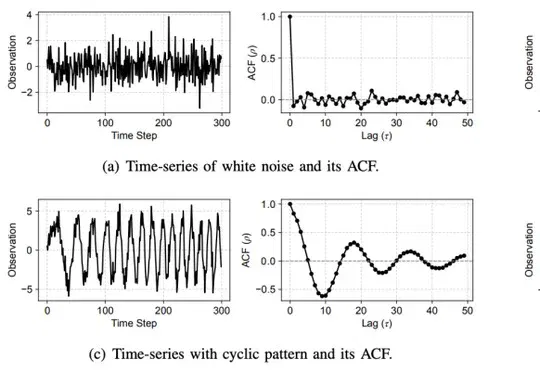
In time series, observations of the same variable at different times are often related. This autocorrelation is an important feature distinguishing time series from ordinary tabular data. For example, today's temperature is usually related to yesterday's. As Figure 1 shows, different time-series patterns correspond to different autocorrelation structures. Effectively modeling this autocorrelation structure is the key to time-series forecasting.
In the statistical-modeling era, classical methods such as ARIMA already modeled autocorrelation explicitly through lag terms. The challenge remains in the deep-learning era: autocorrelation exists both in the historical sequence used as input and in the future sequence used as supervision. Starting from autocorrelation, the survey therefore organizes time-series forecasting around two key questions:
- How should backbone architectures be designed to model autocorrelation in input sequences?
- How should loss functions be designed to model autocorrelation in label sequences?
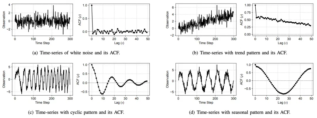
Figure 1: Common time-series patterns and their autocorrelation functions. Trending series usually show strong positive correlation; periodic series alternate between positive and negative correlation as the lag changes; seasonal series often have prominent peaks at integer multiples of the seasonal period.
2. A taxonomy centered on autocorrelation modeling
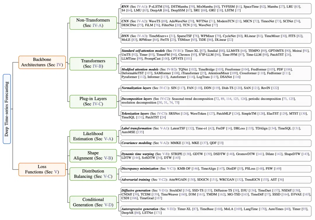
Figure 2: A classification of the literature around autocorrelation modeling.
The figure above shows the survey's framework for classifying the literature. Its first level divides into two main lines, backbone architectures and loss functions, corresponding to the two key questions above. The second level further subdivides methods by their specific modeling approach. The two main lines receive roughly equal space, and both center on autocorrelation modeling, but their objects of focus differ: backbone architectures focus on input sequences (X), while loss functions focus on label sequences (Y). This framework provides a unified perspective for tracing the evolution of both types of method in the sections that follow.
3. The backbone-architecture taxonomy:
Modeling autocorrelation in input sequences
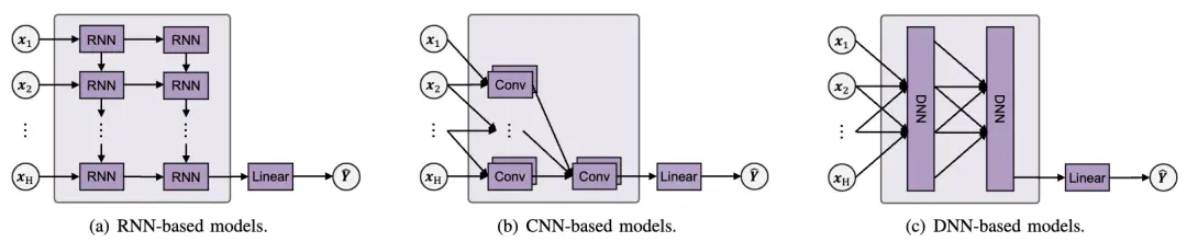
Figure 3: Overview of representative non-Transformer architectures.
The survey first reviews traditional forecasting models.
RNNs' sequential state updates limit parallelism along the time dimension, and finite-dimensional states also limit retention of historical information. Selective state-space models such as Mamba improve efficiency through implementations such as scans, while HiPPO provides a projection-based memory mechanism for continuous signals. These mechanisms do not guarantee that finite-dimensional states preserve arbitrary histories without loss.
CNNs were initially used mainly for image processing. When applied to time series, one-dimensional convolutions aggregate information from neighboring time points to capture local autocorrelation. However, a single standard convolution layer has a limited receptive field. Capturing historical information over longer spans therefore became a focus of later methods. One class of methods expands effective receptive fields in the time domain to cover longer histories, for example through dilated convolutions and large-kernel separable convolutions, increasing coverage while controlling computational overhead. Another class obtains input representations by filtering in the frequency domain, as in FiLM and FilterNet. Under the convolution theorem, frequency-domain filtering is equivalent to time-domain convolution with a full receptive field.
DLinear demonstrated the effectiveness of simple linear models, achieving performance comparable to complex models on some benchmark tasks. However, linear mappings struggle to fully capture nonlinear, nonstationary and interwoven multi-period autocorrelation. Later methods developed in two main directions around this limitation. One transforms data to make modeling easier: DLinear separates components through decomposition and handles them individually, while RLinear uses normalization to mitigate distribution changes. The other enhances model expressiveness: TiDE and TSMixer introduce MLPs to model nonlinearity, and TimeMixer further improves expressiveness through multiscale modeling.
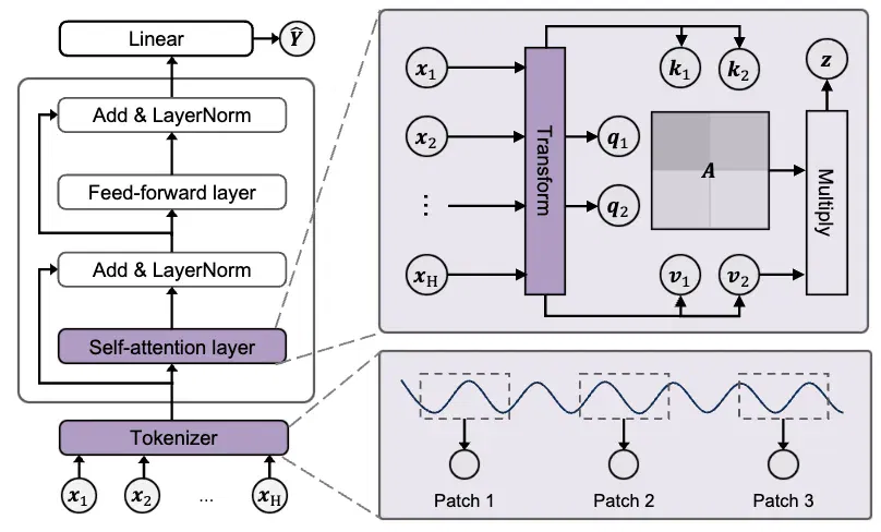
Figure 4: Overview of representative Transformer architectures. Circular nodes represent model inputs and outputs, while colored blocks indicate the main modifications that adapt Transformers to time-series forecasting.
The survey then organizes Transformer-based forecasting models. Transformers use self-attention to model autocorrelation, but directly using observations at individual time points as input often fails to represent temporal semantic information adequately. For example, a temperature value alone provides limited information; changes at neighboring times are needed to determine whether it belongs to a warming trend or a short-term anomaly. To address this, a tokenizer groups consecutive time steps into one token, giving the model local context before it learns long-term dependencies between segments. This design later became almost standard in Transformer time-series models.
Building on this, researchers asked: can the powerful sequence-modeling ability of LLMs be used to model time-series autocorrelation? To do so, the representation of the input sequence must be aligned with the LLM's input representation. The survey identifies four alignment paradigms: the querying paradigm rewrites time-series information as text prompts and uses large language models directly for forecasting, but performance is limited by the ability to express numerical information; the reprogramming paradigm maps time-series segments into the word-embedding space, achieving adaptation without fine-tuning the LLM; the fine-tuning paradigm adapts a pretrained model to time-series data by updating a small number of parameters; the pretraining paradigm directly trains specialized foundation models on large-scale time-series data, such as Timer-XL and Chronos, demonstrating zero-shot forecasting capabilities.
4. The loss-function taxonomy:
Modeling autocorrelation in label sequences
Most existing surveys treat loss functions as implementation details and mention them only briefly. This survey points out that loss functions determine the direction of optimization during model training and deserve attention too. The issue is especially prominent in time-series forecasting: future time points are not isolated from one another, and whether a loss function can effectively model label-sequence autocorrelation is an important challenge. Take mean squared error, or MSE: it calculates prediction errors point by point and aggregates them. Under a probabilistic interpretation, if errors at different forecast steps are further assumed to be mutually independent, minimizing MSE is equivalent to maximizing likelihood. Once the label sequence is autocorrelated, however, that independence assumption no longer holds, and MSE is a biased loss relative to the true likelihood function. How to model label-sequence autocorrelation in a loss function is therefore a distinctive problem in time-series forecasting. Existing methods addressing it can be organized into four classes.
Label transformations seek to calculate error in a more suitable representation space. PCA whitening decorrelates according to the estimated covariance. The effect of a Fourier transform depends on conditions such as the sequence and its boundaries; it does not guarantee complete decorrelation of arbitrary label sequences.
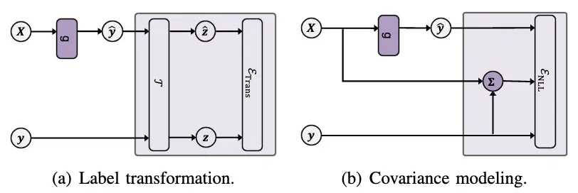
Figure 6: Computation of a loss function based on likelihood estimation
The second class constructs losses through shape alignment. Its basic assumption is that autocorrelation is reflected in the waveform of the label sequence, so the loss should focus on whether predicted and true waveforms match, rather than the magnitude of pointwise errors. DTW is a classical method for measuring waveform differences, but it is not differentiable and cannot be used directly for gradient optimization. SoftDTW applies a soft relaxation to DTW, producing an everywhere-differentiable loss that supports end-to-end training. These losses are especially effective where phase invariance is needed. For example, in ECG signals, a prediction that lags by half a beat overall but has the correct waveform shape is still much more valuable than one with a distorted shape.
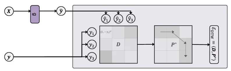
Figure 7: Computation of a loss function based on shape alignment
The third class constructs losses through distribution alignment. Its core idea is that autocorrelation is reflected in the label sequence's conditional distribution. A loss that brings the conditional distributions of the predicted and label sequences closer together can therefore incorporate label autocorrelation into the training objective. The key is how to construct the distance between probability distributions. Existing approaches fall into two groups. One directly uses an existing distribution distance as the loss: DistDF uses Wasserstein distance, for example, while KMB-DF uses MMD distance. The other draws on adversarial learning to learn the distribution distance adaptively, training a discriminator so it cannot distinguish predicted sequences from label sequences, thereby achieving distribution alignment.
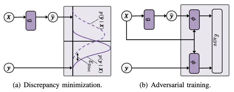
Figure 8: Computation of a loss function based on distribution balancing
The fourth class constructs losses through conditional generation. These methods no longer directly regress future values. Instead, they treat forecasting as a generation task and use a generative model's inference mechanism to model autocorrelation. There are two specific routes. One, represented by CSDI, is diffusion generation, which generates future sequences through progressive denoising. The other, represented by DeepAR, is autoregressive generation, where each generation step depends on earlier outputs, explicitly decomposing the future into a chain of dependencies. The core advantage of conditional generation is that it fundamentally avoids autocorrelation bias: the generation process itself assumes a sequential dependency structure, without needing to introduce an independence assumption as MSE does.
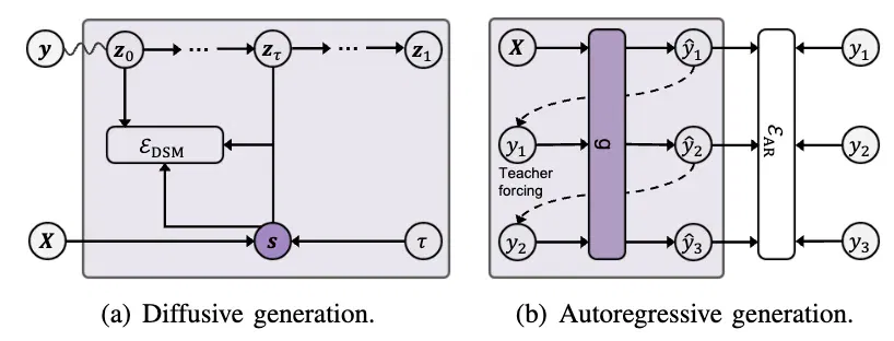
Figure 9: Computation of a loss function based on conditional generation
5. Outlook for research on autocorrelation modeling
The review above shows that autocorrelation modeling is an important thread running through time-series forecasting research, driving the proposal and improvement of many methods. On this basis, the survey looks ahead to future research in four areas; two are listed here:
First, address the challenges of autocorrelation modeling in real settings. Real time-series data often contain measurement noise, distribution shifts and missing observations. For measurement noise, one could explore denoising learning for continuous labels; for distribution shift, techniques such as domain adaptation, domain generalization and test-time adaptation could be introduced to balance responsiveness to distribution changes with robustness. For missing observations, a common practice is to impute first and forecast afterward, but imputation errors can distort temporal structure and thereby affect forecast quality. Thus, directly forecasting from incomplete observations and fusing data with multiple sampling rates also deserve research.
Second, transfer autocorrelation-modeling methods to modeling dependencies between variables. In multivariate forecasting, correlations between different variables or channels also affect performance. The vast majority of methods used to model autocorrelation, such as self-attention and label transformations, can be extended directly to the variable dimension; considerable research space remains for designing network architectures and loss functions that simultaneously capture autocorrelation and dependencies between variables.
Conclusion
In recent years, forecasting models have developed rapidly and new methods have continued to emerge. Through the unified perspective of autocorrelation modeling, the survey attempts to answer two connected questions: What are the core challenges of deep time-series forecasting, and how do existing methods address them? Autocorrelation is no longer an abstract term in statistics textbooks, but an important object that must be modeled when designing forecasting methods in the deep-learning era. Whether designing better architectures or constructing more appropriate loss functions, the same question is unavoidable: have we better understood and modeled the intrinsic dependency structure of time series? Understanding and modeling autocorrelation has always been a distinctive feature and core problem of this field.
Author team
The corresponding authors are Professors Haoxuan Li and Zhouchen Lin (IEEE Fellow) of Peking University. The work was completed jointly with institutions including the University of Southern California, Zhejiang University, the University of Oxford, the University of Melbourne, Squirrel AI and Xiaohongshu. This work received strong support from the Beijing Municipal Science and Technology Commission and the Administrative Commission of Zhongguancun Science Park. We express our sincere gratitude!
This article comes from the WeChat public account Synced and was written by Synced.
Related topics
After reading
Join the AINRK community
Read how to join the community and connect with people working in AI.
Related articles
Continue reading related topics and articles in this category.
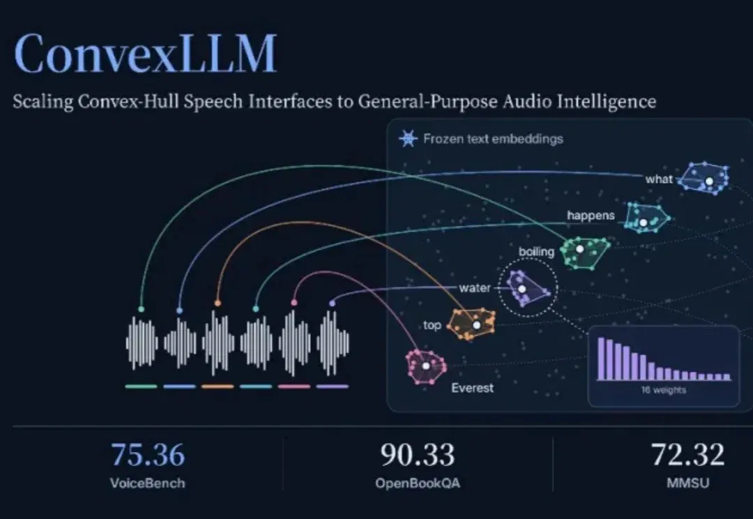
ConvexLLM connects speech to language models through frozen text embeddings (opens in a new tab)
Researchers at CUHK-Shenzhen and Microsoft propose C-Gate, mapping audio into convex combinations of frozen text embeddings. The paper reports VoiceBench gains against its listed open-model baselines, while audio understanding and transcription still involve trade-offs.
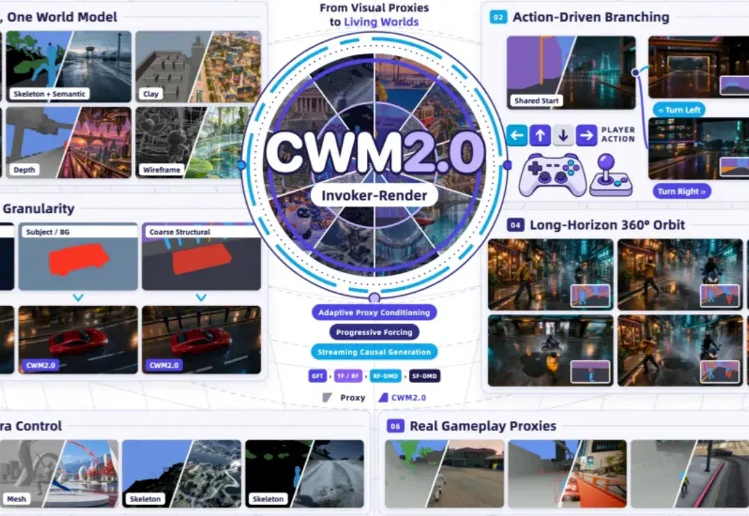
CWM2.0 open-sources generative rendering with a 30-minute racing demo (opens in a new tab)
Teams from Ant, Westlake University and Zhejiang University use a structured Proxy to control scene state and Invoker-Render to generate visuals, releasing eight-GPU streaming inference. The long demo and 140 evaluations cover specified scenes, not arbitrary stable worlds.
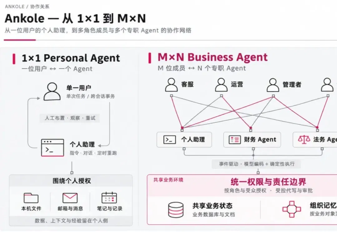
Ankole outlines multi-user agent architecture: events, permissions and organizational memory (opens in a new tab)
The team describes its Business Harness design for fast and slow paths, shared state, Actor orchestration and dynamic permissions. Formal verification covers the modeled core permission state machine; it does not replace security checks of the full deployment, external interfaces or implementation.
openJiuwen presents a Harnessless approach for reusing AgentOS execution tools (opens in a new tab)
openJiuwen uses app-development and swarm demos to show how built-in harness capabilities support sessions, tools and app management. Applications still define business rules and permissions; remote deployment and some capabilities remain planned or exploratory.
Ask-to-Distill optimizes training questions using teacher–student distribution signals (opens in a new tab)
UIUC and collaborators propose A2D, training a question generator with frozen teacher–student disagreement and compatibility signals before on-policy distillation. The paper reports gains in math, code and agent tasks; its learning-value proxy has limits.